The setting
A great many problems in science and engineering reduce to the same template: we observe a system at a handful of moments in time, and we want to recover the underlying rule that drives it. Population sizes, the swing of a pendulum, climate variables, the chemistry of a reactor — all of these are modeled by a dynamical system, written compactly as $\dot{x}(t) = f(x(t))$. The standard recipe is to pick a flexible family of candidate $f$'s — neural networks (the “neural ODE” approach), sparse dictionaries, polynomials, Gaussian processes, you name it — and then to tune the parameters of $f$ so that predictions match the observations. The most popular instance of this template today, by far, is the neural ODE: $f$ is a neural network, the parameters are its weights, and the loss compares predicted samples to observed ones at the data times.
But here is the catch that this paper is about: to compare a candidate $f$ to data, the training loop has to simulate $f$ forward in time, and that simulation requires a numerical integrator. Forward Euler. Runge–Kutta. Implicit midpoint. Whichever method you reach for becomes silently stitched into the loss function. Different integrators give different losses, and therefore prefer different $f$'s. The result is that the integrator can shape, and sometimes mis-shape, what you learn — whether your $f$ is a neural network with a million parameters or a three-coefficient polynomial.
What is the trained model used for?
Before we dig into the artifact, it is worth being explicit about why a reader should care. Once a candidate $\hat f$ has been fit, it gets used in one of two qualitatively different ways:
- To understand the rule. The trained $\hat f$ is itself the object of interest — one inspects it as a continuous-time differential equation $\dot x = \hat f(x)$ and reads off scientific structure from it: equilibria and their stability, conserved quantities, growth or decay rates, oscillation frequencies, sensitivities to parameters. This is the “equation discovery” or “system identification” usage: what law is the data obeying? Here the qualitative properties of $\hat f$ are the deliverable, and getting the sign of dissipation wrong is a fatal error.
- To simulate further. The trained model is used as a discrete dynamical system — the integrator $S_h[\hat f]$ at the training step $h$ — to roll the state forward beyond the observation window, perhaps from new initial conditions, perhaps over longer horizons, perhaps as a fast surrogate inside a control or design loop. This is the forecasting / surrogate-modeling usage: what will the system do next? Here the deliverable is predicted trajectories rather than the form of $\hat f$.
These two usages are not equally robust to integrator artifacts. Usage (1) is fragile: the analysis below shows that the integrator inside the training loop can flip the sign of $\mathrm{Re}\,\hat\lambda$ in the linearization of $\hat f$, so any conclusion drawn from the continuous-time form of $\hat f$ may be qualitatively wrong. Usage (2) looks safer at first — if you keep using the same integrator at the same step $h$, the discrete predictions $S_h^n[\hat f]\, y_0$ are well-fit to the training data — but it stops being safe the moment you change the simulation step, switch integrators, or run from initial conditions outside the training set, all of which the demos below illustrate. In short, the integrator artifact eventually bites both usages, just at different moments.
The optimization problem
It will help to make the training problem explicit, in a form general enough to cover neural ODEs, sparse regression, kernel models, and any other trajectory-fitting setup — not just the linear scalar special case we will analyse afterward.
Suppose we observe a system at a finite collection of times. We sample the true trajectory at evenly spaced moments $t_n = n H$, for $n = 0, 1, \ldots, N$, possibly starting from $M$ different initial conditions $y_0 \in U_M$. The dataset is
\[ \mathcal{D}_N \;=\; \big\{\, \bigl(t_n,\; y(t_n; y_0)\bigr)\,:\, n = 1, \ldots, N,\; y_0 \in U_M \,\big\}. \]We choose a function class $\mathcal{F}$ — the class of neural networks with a chosen architecture, the span of a sparse dictionary of candidate terms, a reproducing kernel Hilbert space, or anything else — and we look for the $\hat f \in \mathcal{F}$ whose flow best reproduces the data. Idealised, that means
\[ \min_{\hat f \in \mathcal{F}}\; \frac{1}{N M}\,\sum_{y_0 \in U_M}\sum_{n = 1}^{N}\, \bigl|\,\phi_{t_n}[\hat f]\, y_0 \;-\; y(t_n;\, y_0)\,\bigr|^{2}, \]where $\phi_{t}[\hat f]\, y_0$ is the exact continuous-time flow of $\dot x = \hat f(x)$ from $y_0$ to time $t$. This is the form of the problem people imagine they are solving when they write a neural-ODE training loop.
But the exact flow $\phi_t[\hat f]$ has no closed form for a generic $\hat f$, so the training loop has to approximate it. Pick a numerical integrator, call its one-step propagator $S_h[\hat f]$, and replace the exact flow by repeated application of $S_h$:
\[ \min_{\hat f \in \mathcal{F}}\; \frac{1}{N M}\,\sum_{y_0 \in U_M}\sum_{n = 1}^{N}\, \bigl|\,S_h^{m n}[\hat f]\, y_0 \;-\; y(t_n;\, y_0)\,\bigr|^{2}, \qquad m h = H. \]This is the problem actually solved by the optimizer. Now $S_h[\hat f]$ — whether forward Euler, classical RK4, the implicit midpoint rule, Leap Frog, or anything else — is welded into the loss function. Different choices of $S_h$ produce different losses, and therefore different global minimizers $\hat f$. The minimizer of this second problem can differ from the minimizer of the first by a lot, and this paper is about exactly how it differs and what to do about it.
The rest of the page concentrates on the simplest case in which the gap between the two problems is unambiguous: a one-dimensional linear scalar $\dot z = \lambda z$. Even there, the integrator can move the inferred $\hat\lambda$ across the imaginary axis — flipping the sign of damping — without leaving any sign of trouble in the loss value. That is the cleanest possible example of a much more general phenomenon: the integrator is part of the model.
A surprise: damped becomes anti-damped
The cleanest way to see the trouble is with a system whose true behavior is uncontroversial. Take a damped oscillator in the plane:
\[ \dot{x} = -\alpha\, x - \omega\, y, \qquad \dot{y} = \omega\, x - \alpha\, y. \]With $\alpha > 0$ this spirals inward toward the origin — classic damping. Now sample its trajectory at evenly spaced times, hand those samples to a training loop, and ask the loop to recover the underlying linear dynamics. The training loss is the difference between the observed samples and the predictions made by the integrator at the training step $h$. Many different continuous-time $\hat A$ can give zero loss: any $\hat A$ for which the integrator's discrete iteration at step $h$ lands on the data dots. For classical RK4 there are four such $\hat A$ for a generic $h$. Some of them have negative damping. Some rotate in the opposite direction. They are global minima of the training loss, every bit as valid to the optimizer as the truth.
The illustration above the abstract makes this concrete. We sampled a damped oscillator at evenly spaced times (the black dots), then asked an RK4-based optimizer to fit a continuous-time $\hat A$. With the step size set to $h = 1.0$, the optimizer settled on a $\hat A$ whose four candidate eigenvalues include $\hat\lambda \approx 0.105 + 1.927i$ — positive real part. The green curve is RK4 at the training step $h$ run on this $\hat A$; it passes exactly through the data, and from inside the training loop nothing is amiss. The red curve is RK4 at step $h/100$ on the very same $\hat A$ — close enough to the exact flow that what you see is what the learned ODE genuinely does. It spirals outward.
Even forward Euler, which has only a single candidate $\hat\lambda$, can land far from the truth: the recovered system stays damped, but with a decay rate much larger than the truth's. The same green-vs-red trick exposes that artifact too — you can watch it happen below.
Try it: shrink the simulation step $\tilde h$ and watch the learned ODE reveal itself
The training step is fixed at $h = 1.0$, exactly as in the figure above the abstract. The optimizer fits a continuous-time $\hat A$ so that the chosen integrator at step $h$ reproduces the data dots. The green trajectory is exactly that fit. The red trajectory uses the same integrator on the same $\hat A$, but with a smaller step $\tilde h$. As $\tilde h$ shrinks, the integrator becomes more and more accurate — in the limit it is the exact flow of the learned ODE. So as you drag $\tilde h$ down from $h$, the red curve peels away from the green one and reveals what the learned ODE is actually doing.
Where does the artifact come from?
Every numerical integrator turns the continuous-time question “given $f$, where is the trajectory at time $t+h$?” into a discrete map of the form $x_{n+1} = R(hA)\, x_n$, where $A$ is the local linearization of $f$ and $R$ depends on the integrator. Forward Euler chooses $R(z) = 1 + z$. Classical RK4 chooses $R(z) = 1 + z + z^2/2 + z^3/6 + z^4/24$. The implicit midpoint method chooses $R(z) = (2+z)/(2-z)$.
Each $R$ has a stability region in the complex plane: the set of values $z$ for which $|R(z)| \le 1$, so that the discrete iteration decays rather than blows up. When you train a model from sampled data, the optimizer is essentially solving an inverse problem on $R$. For the trajectory to decay the way the data does, the optimizer needs the product $h \lambda(\hat A)$ — where $\lambda(\hat A)$ runs over the eigenvalues of the learned dynamics — to land inside the stability region. And here is the trap: parts of these stability regions can lie in the right half complex plane, where $\mathrm{Re}\,\lambda > 0$. A positive real part is the mathematical signature of anti-damping.
Try it: where do the stability regions live?
The shaded area is the stability region of the chosen integrator. Decay of the discrete map is guaranteed inside it. The blue dot is $h\lambda$ for the true (damped) system. As $h$ grows, blue can drift out of the stability region; the training loop responds by moving $h\lambda(\hat A)$ — the red dot — back inside. Notice how often the only way for it to do that is to cross into the right half plane.
Why a smaller step size is not always the answer
The first instinct of any numerical analyst, when something looks unstable, is to shrink $h$. That works in this setting too — eventually. But “eventually” can be costly, because the data is only sampled every so often, and small $h$ means many integrator steps between observations.
The second instinct is to switch to a higher-order explicit integrator, such as RK4. The hope is that more accurate per-step prediction will mean less artifact. The opposite turns out to be true in general. The stability regions of explicit Runge–Kutta methods bulge further into the right half plane as the order increases. So a higher-order explicit integrator gives the optimizer more room to land on a learned $\hat A$ with positive real part — that is, more anti-damped solutions look acceptable, not fewer. You can see this in Demo 2 above: switch from forward Euler to RK4 and watch the right-half-plane lobe grow.
The principled fix: use a structure-preserving integrator
The implicit midpoint method has a stability region equal to the entire closed left half plane. Stable continuous dynamics — those with $\mathrm{Re}\,\lambda \le 0$ — map to stable discrete dynamics, and unstable to unstable. Nothing crosses sides. As a consequence, when implicit midpoint is used inside the training loop, the qualitative character of the data is preserved: a damped oscillator stays damped under the learned model, and a conservative system stays conservative. This holds even when the only prior information about the system is that it is autonomous — no special knowledge of energy, dissipation, or symplectic structure is needed in advance.
Try it: forward Euler vs. implicit Euler vs. implicit midpoint, side by side
Same data on all three panels. On each panel the green curve is the integrator at step $h$ applied to the learned $\hat A$ on that side (it sits on the data, by construction); the red curve is the same integrator at step $h/100$ on the same $\hat A$ (a near-exact rendering of the learned ODE). Three integrators, three artifacts: forward Euler over-decays (left), implicit Euler over-grows (centre), implicit midpoint stays faithful (right).
Multi-step methods: a parasitic mode lying in wait
Everything above involved one-step integrators — methods that compute the next state from just the current one. Many widely used schemes are multi-step: they advance using the last several states. The classical Leap Frog scheme is the simplest example, $\;z_{n+1} = z_{n-1} + 2h\, \hat\lambda\, z_n$. It is two-step, second order, and it is everywhere — molecular dynamics, plasma simulations, structured Hamiltonian solvers, parts of every introductory PDE course.
A two-step recurrence has two characteristic roots for each true eigenvalue. For Leap Frog applied to the data of a damped oscillator, the optimizer ends up using $\hat\lambda = \sinh(h\lambda)/h$, and the recurrence has roots $\zeta_+ = e^{h\lambda}$ (the “physical” mode that decays in step with the data) and $\zeta_- = -e^{-h\lambda}$ (a “parasitic” mode that grows by a factor $e^{h\alpha}$ each step). Their product is fixed at $\zeta_+ \zeta_- = -1$, so whenever the physical mode decays, the parasitic one grows by exactly the same factor.
When the leap-frog iteration starts from the same initial conditions $(z_0, z_1)$ that the data was generated from, the parasitic mode has coefficient zero and stays silent forever. Change the initial conditions even slightly — perturb $z_1$ by a small amount — and the parasitic mode wakes up. Once awake, it dominates the trajectory exponentially.
Try it: a tiny perturbation in $z_1$ wakes up the spurious root
Same data, same learned $\hat\lambda$. The green curve is Leap Frog started from the data's own initial pair $(z_0, z_1)$ — only the physical root is excited, and the trajectory hugs the data and its continuation indefinitely. The red curve starts from the same $z_0$ but with $z_1$ shifted by $\varepsilon$ in the real direction. As you increase $\varepsilon$ from $0$, the red trajectory starts to break away from the data and eventually diverges — that's the parasitic mode showing up. Increase the perturbation, or watch later in time, to see how strongly it dominates.
This is the qualitative difference between one-step and multi-step methods in the learning context. With a one-step integrator the artifact lives in $\hat\lambda$ itself. With a multi-step integrator, $\hat\lambda$ may be exactly faithful to the training data, yet the resulting discrete model has a parasitic root that any nontrivial perturbation of the initial state can ignite. In practice such perturbations are unavoidable: they come from measurement noise, from bringing the model to a slightly different starting condition, from any mismatch between training-time and deployment-time initial data.
The same artifact in a nonlinear system: Lotka–Volterra
Everything above was the linear scalar problem — the simplest setting in which the artifact can be analyzed cleanly. To see that the same mechanism shows up in real nonlinear systems trained with neural ODEs, the paper runs the experiment on the textbook predator–prey model first written down by Lotka and Volterra in the 1920s.
The Lotka–Volterra equations describe how a population of prey $x$ and a population of predators $y$ feed back on each other:
\[ \dot x \;=\; \alpha\, x \;-\; \beta\, x y, \qquad \dot y \;=\; \delta\, x y \;-\; \gamma\, y. \]Each prey individual reproduces at rate $\alpha$ and is eaten at rate proportional to the predator population. Each predator dies at rate $\gamma$ and is born at rate proportional to how many prey it can find. With positive constants $\alpha, \beta, \gamma, \delta$, the system has one non-trivial equilibrium where birth and death exactly balance, and every other trajectory traces a closed loop in the $(x, y)$ plane around that equilibrium — populations cycle forever, prey rising then predators rising then prey falling then predators falling. The loops never spiral in and never spiral out. The system is conservative: it has an exactly preserved quantity (a generalised energy) along every orbit.
That makes Lotka–Volterra a particularly clean test for the integrator-induced artifact. There is no “true” damping the optimizer could discover — the right answer is closed orbits and nothing else. So if the trained model produces a trajectory that spirals inward, that spiral is entirely an integrator artifact; there is no dissipation in the data to fit.
In the experiment from the paper, three Lotka–Volterra trajectories — three nested closed orbits — are sampled at evenly spaced times and used to train a neural-network vector field. The training fit at the sample points is excellent in every case. But running the learned vector field with a fine-step integrator (essentially the exact flow) tells three very different stories depending on which integrator was inside the training loop.
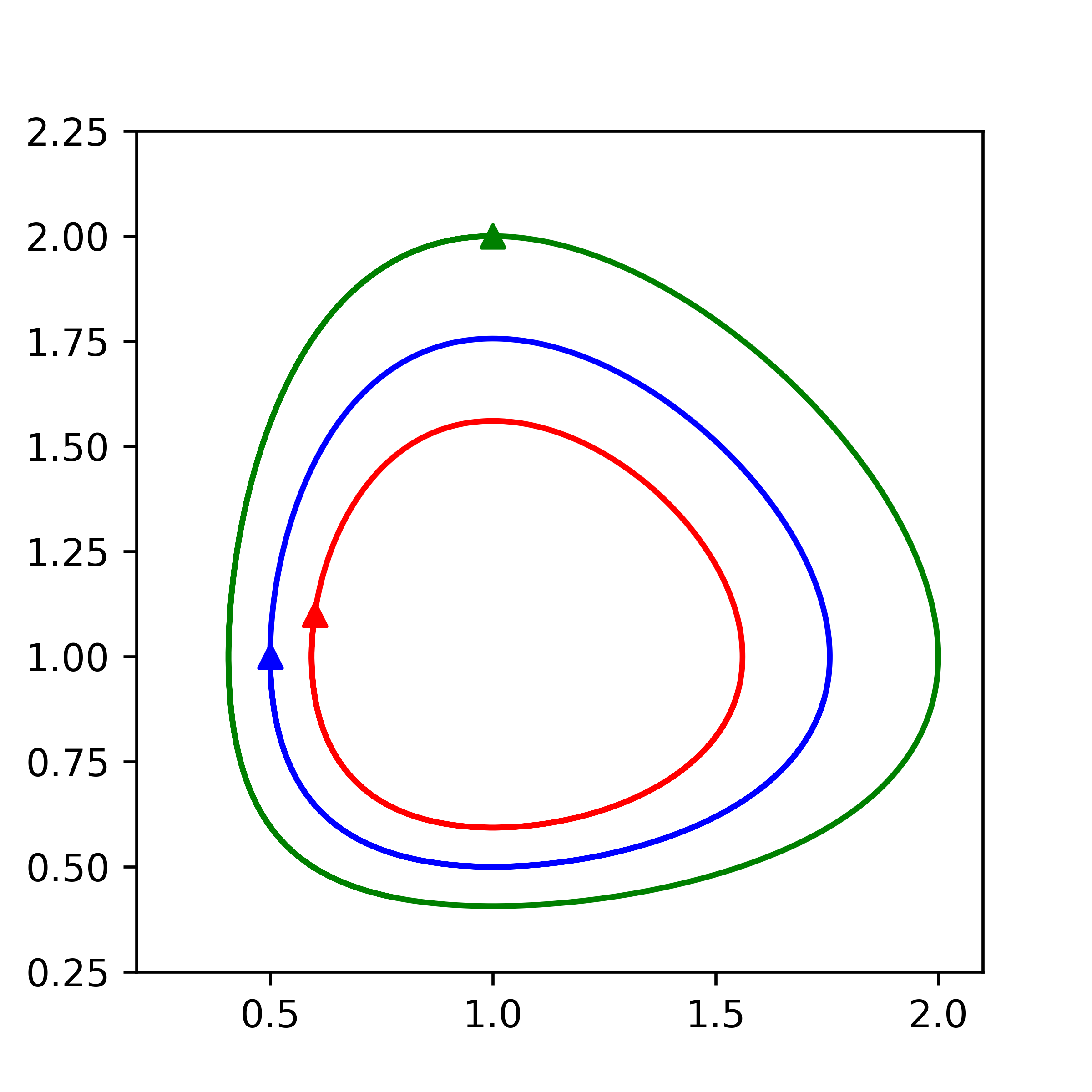
Truth: three closed predator–prey orbits in the $(x, y)$ phase plane. Populations cycle indefinitely with no decay.
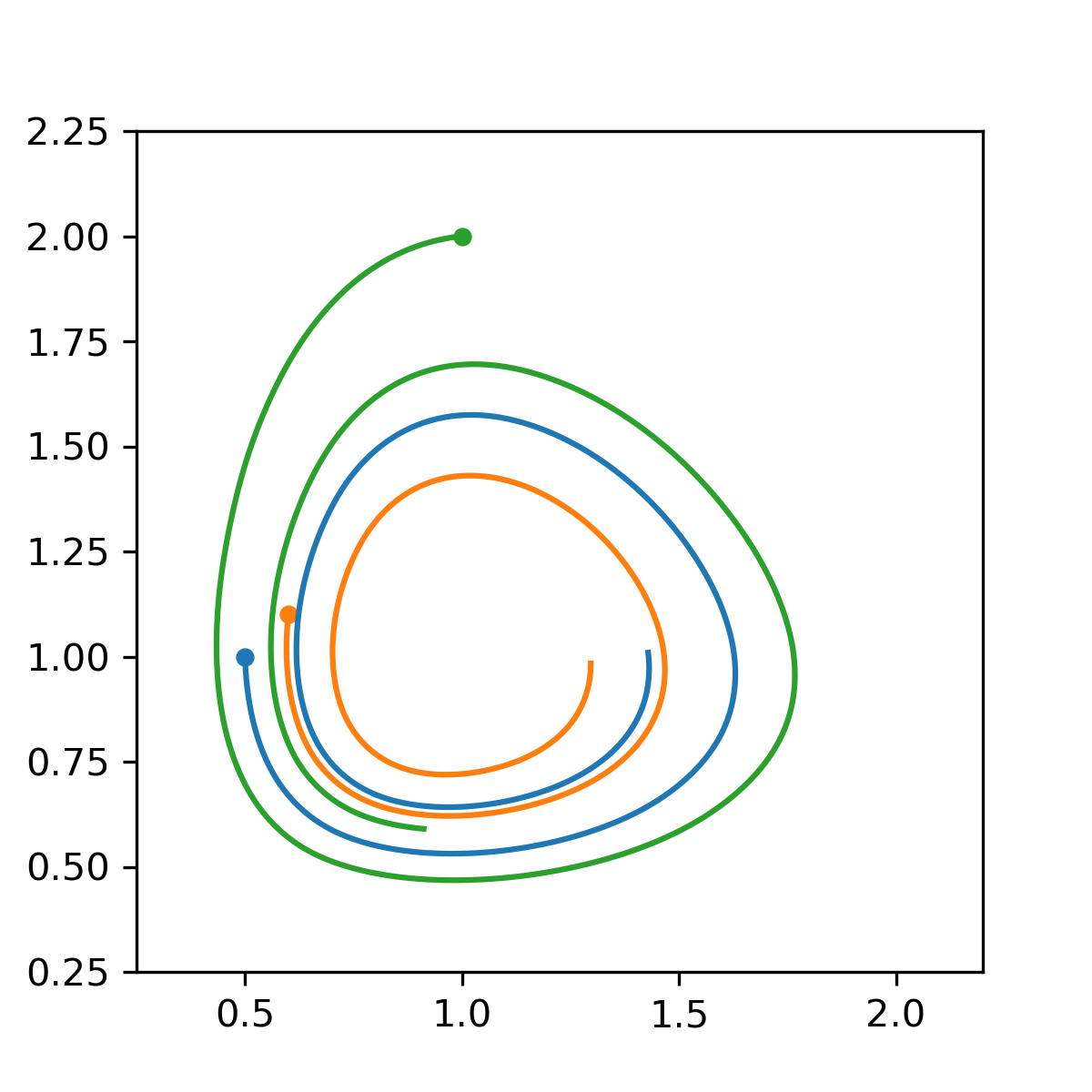
Learned with RK4: the same three initial conditions, integrated with the learned vector field at fine resolution, spiral inward toward equilibrium — a non-physical dissipation that came from the integrator, not the data.
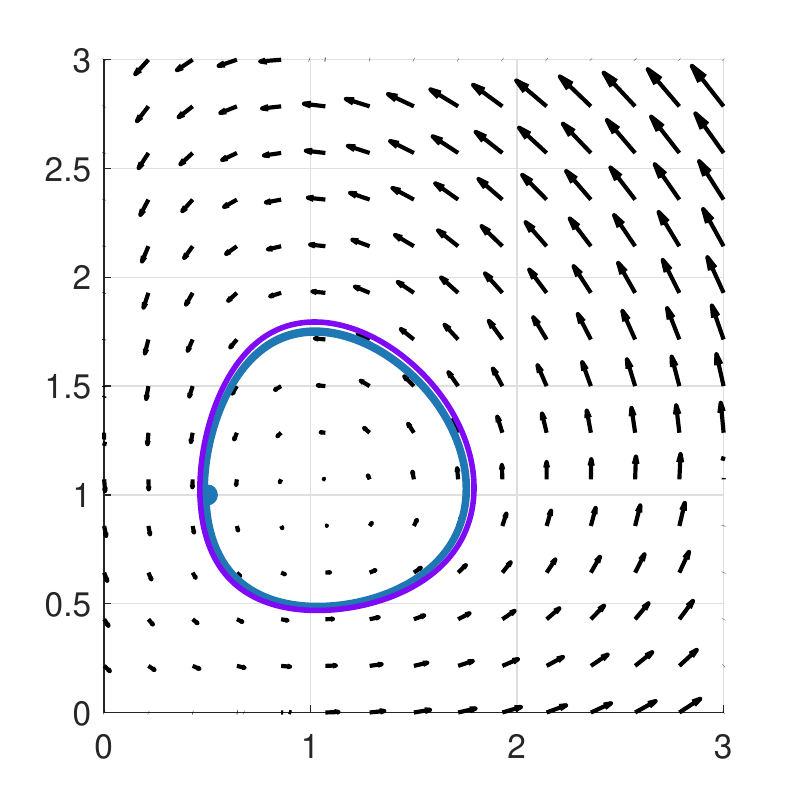
Learned with implicit midpoint: the learned vector field (arrows) and a high-resolution trajectory (purple) sitting almost exactly on the true closed orbit (blue). The conservative structure is preserved.
What this means in practice
If you build models of physical or scientific systems from time-sampled data — whether you call the model a neural ODE, a SINDy-style sparse regressor, a Gaussian process flow, or anything else — the integrator inside your training loop is part of your model class. It comes with biases, and for autonomous systems those biases can flip the sign of damping or the direction of rotation without flagging a single warning.
Two practical takeaways follow:
- Treat the integrator as a modeling choice, not a default. Document which integrator and which step size you used, just as you would document your loss function or your network architecture.
- Prefer a numerical integrator whose stability region is exactly the left half complex plane. That is the geometric criterion the analysis in this paper points to: when the stability region coincides with $\{z : \mathrm{Re}\, z \le 0\}$, the learned eigenvalues automatically inherit the correct sign of dissipation from the data, without any structural prior beyond autonomy. Among classical methods, the implicit midpoint rule satisfies this exactly; it is a safe default when the only thing you know about the system is that it is autonomous.
We are pursuing these questions in the Scientific AI Research Group at the Oden Institute and the Department of Mathematics at UT Austin, where much of our work sits at the boundary where numerical analysis impacts deep learning practices: characterising how classical numerical methods shape what data-driven models can and cannot represent, and using that understanding to design training pipelines that learn more reliably. The conviction running through the group is that numerical analysis can help bring more effective learning to data-driven models of dynamical systems — and that the integrator choice studied in this paper is just one of several places where that contribution is concrete.
Reference
Bing-Ze Lu and Richard Tsai. Artifacts of Numerical Integration in Learning Dynamical Systems. arXiv:2507.14491 [math.NA / cs.LG], 2025. [PDF]