Abstract
Sensor placement optimization methods have been studied extensively. They can be applied to a wide range of applications, including surveillance of known environments, optimal locations for 5G towers, and placement of missile defense systems. However, few works explore the robustness and efficiency of the resulting sensor network concerning sensor failure or adversarial attacks. This paper addresses this issue by optimizing for the least number of sensors to achieve multiple coverage of non-simply connected domains by a prescribed number of sensors. We introduce a new objective function for the greedy (next-best-view) algorithm to design efficient and robust sensor networks and derive theoretical bounds on the network's optimality. We further introduce a Deep Learning model to accelerate the algorithm for near real-time computations. The Deep Learning model requires the generation of training examples. Correspondingly, we show that understanding the geometric properties of the training data set provides important insights into the performance and training process of deep learning techniques. Finally, we demonstrate that a simple parallel version of the greedy approach using a simpler objective can be highly competitive.
Introduction
In the multi-coverage sensor placement problem the goal is to compute optimal sensor locations such that the majority of the free space is observed by at least \( k \) sensors. For this we assume that an environment \( \Omega \) consists of regions occluded by obstacles \( \Omega_\text{obs} \) and free space \( \Omega_\text{free} \).
A point \( x \in \Omega_\text{free} \) is visible to another point \( y \in \Omega_\text{free} \) if there is an unobstructed straight line between them.
\[ \mathbf{x} \overset{\text{vis}}{\sim} \mathbf{y} \iff \forall t \in [0,1] \text{: } t\mathbf{x} + (1-t)\mathbf{y} \in \Omega_\text{free}. \]
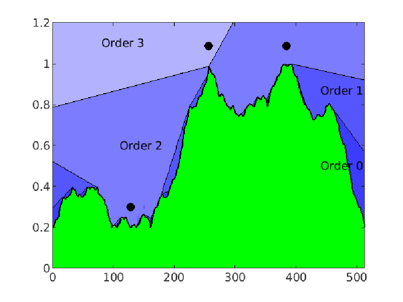
The order of visibility function \( \mathcal{O}_\text{vis} \) returns the number of sensors in a set of sensor \( P \) that observe a given point.
\[ \mathcal{O}_\text{vis}(\mathbf{y}; P) = \sum_{x \in P} \phi_{\mathbf{x}}(\mathbf{y}) \]
where
\[ \phi_{\mathbf{x}}(\mathbf{y}) = \begin{cases} 1, & \text{if } \mathbf{x} \overset{\text{vis}}{\sim} \mathbf{y},\\ 0, & \text{else.} \end{cases} \]
The multi-coverage sensor placement problem can then be described as
Multiple coverage optimization:
Find the minimal set of sensors \( P = \{x_1,...,x_n\} \) such that
\[ \text{Vol} \left( \left\{y\in \Omega \vert~ \mathcal{O}_\text{vis}(y; P) \geq k \right\} \right) \le (1 - \delta) \text{Vol}(\Omega_{\text{free}}), \]
for some given threshold \( \delta \in (0,1). \)
Greedy Algorithm
Even the single coverage problem is known to be NP-complete for general environments. To address the challenge of efficient computation of sensor location we relax the problem using the next-best-view principle where sequences of sensors are generated instead of sets. This leads to the development of the \( \epsilon \)-greedy algorithm.
    def eps_greedy_alg(eps, k):
        P = list()
        while Vol(O_vis(P) >= k) <= delta:
            G = compute_objective_G(P, k)
            M = max(G)
            feasible = [x for x in PossibleLocations if G(x) >= (1-eps)*M]
            x = feasible[randint(0, len(feasible))]
            P.append(x)
        return P
This algorithm chooses the next sensor by (somewhat) greedily maximizing a objective function (using function compute_objective_G). In our case the objective function return the gained volume of regions of order up to target order \( k \) by placing a new sensor in a given location.
\[ \mathcal{G}_k(x, P) = \sum_{i=1}^k w_i \int_{\Omega_\text{free}} 1_{\{\mathcal{O}_{\text{vis}}(\mathbf{z}, P \cup \{x\}) \geq i\}} - 1_{\{\mathcal{O}_{\text{vis}}(\mathbf{z}, P) \geq i\}} d\mathbf{z}. \]
Here the integrals descirbe the gain in the volume of regions of order at least \( i \) which are weighted by weights \( w_i \). The weights describe the priority of different orders of visiblity in the algorithm.
To measure the quality of a set of sensors we use a function \( f_k \) closely realted to the objective function \( \mathcal{G}_k \).
\[ f_k(P) = \sum_{i=1}^k w_i \int_{\Omega_\text{free}} 1_{\{\mathcal{O}_{\text{vis}}(\mathbf{z}, P) \geq i\}} d\mathbf{z}. \]
It describes a weighted sum of volumes of regions with specified minimal achieved order. If a region is not observed by any sensor it assigns value \( 0 \). If a region is observed by at least one sensor it assigns value \( w_1 \), if observed by at least two sensors the assigned value is \( w_1 + w_2 \) and so on. This allows us to measure the value of partial coverage and we are able to analyze the quality of the sensor set produced by the greedy algorithm.
Effectivity guarantee
Let \( P_n = \{x_1,...,x_n\} \) be the set of $n$ sensors placed according to the greedy algorithm using \( \mathcal{G}_k \) and parameter \( \epsilon \in [0,1) \).
\[ P_l^* = \{x_1^*,...,x_l^*\}\in \underset{P \subseteq \Omega_\text{free}, \vert P \vert = l}{\operatorname{argmax}} f_k(P) \implies f_k(P_n) \geq \left( 1 - e^{-(1-\epsilon)\frac{n}{l}} \right) f_K(P_l^*). \]
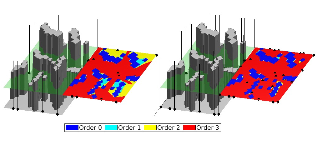
Also for empirical examples the algorithm produces promising results. In the example shown 10 sensor are sufficient to cover 45% of \(\Omega_\text{free}\) with order 3 visiblity (left). After 24 sensors are placed 90% of the free space is observed by at least 3 sensors and the greedy algorithm terminates (right).
Parallel Greedy Algorithm
Another approach we looked at was to split the multi-coverage problem into multiple single coverage problems. Solving the single coverage problem using the greedy algorithm using objective function \( G_1 \) has been expensively studied in the past and promises to be effective. Since practice we want to avoid sensors being placed too close or at the same location, we place the first sensor in each run randomly to introduce variability in the sensor network.
    def par_greedy_alg(eps, k):
        P = list()
        for i in range(k):
            S = eps_greedy_alg(eps, 1)
            P += S
        return P
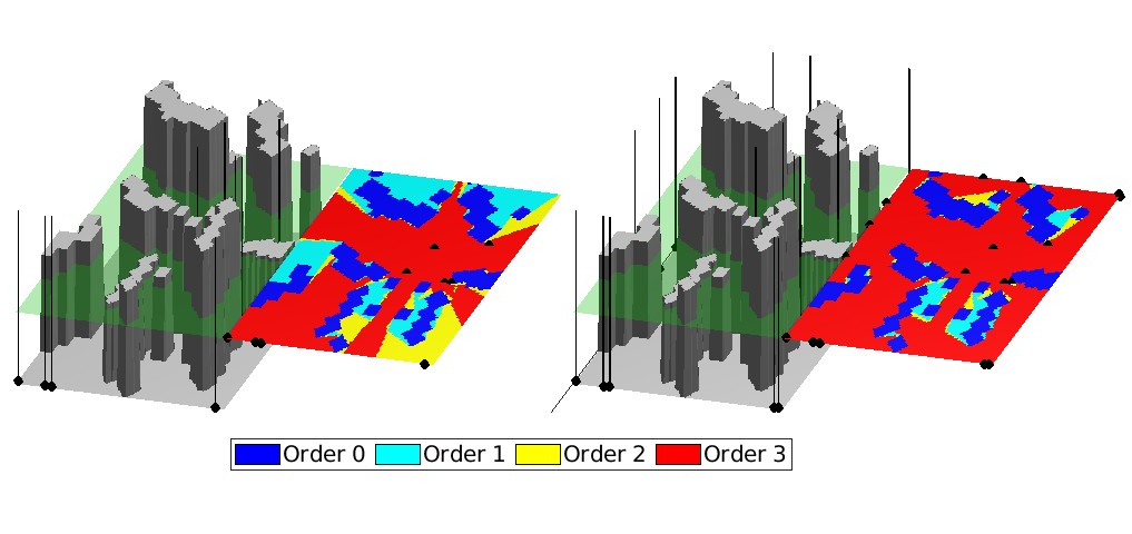
Note that the calculations inside the for loop are independent of eachother and can therefore be performed in parallel which significantly increases the speed. Here 9 sensors were needed to observe 43% of the \( \Omega_\text{free} \) with at least 3 sensors which is slightly worse that the result of the order 3 greedy algorithm. However the termination criterion of 90% observed by at least 3 sensors is reached using only 18 sensors.
Learning the Objective Function using Deep Learning
In the algorithms discussed above the evaluation of the objective function \( \mathcal{G}_k \) and \( \mathcal{G}_k \) is still computationally expensive. We use deep learning techniques to compute approximations of $\( \mathcal{G}_k \) which significantly imporves the speed of the algorithm once trained. In this approach we use the TiraFL network architecture to approximate the objective function \( \mathcal{G}_k \).
\[ \mathcal{G}^\theta_k(x, P, \Omega_\text{free}) \approx G_k(x, P) \]
The approximation of \( \mathcal{G}_1 \) has been discussed in "Visibility Optimization for Surveillance-Evasion Games". To compare the different methods we used 50 sample maps generated by assigning random heights to random crops of Massachusetts building footprints.
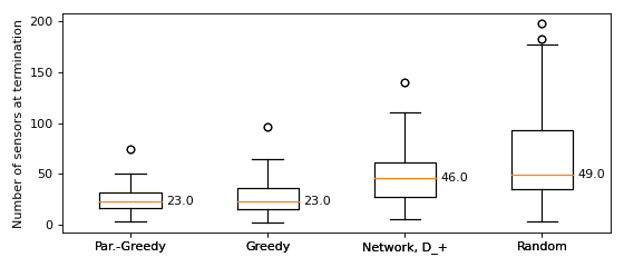
The boxplots illustrate the number of sensor needed to reach the threshold of 90% order 3 coverage. Both the greedy and parallel greedy algorithm are shown to be very effective. The network approximation, while not as effective, still consistently produces good results. As reference we also show the results for random placement of sensors.
Publications